In this chapter we’ll go through checking and cleaning tag detections by by filtering out noisy data, visually exploring your data, and checking ambiguous detections.
Some extra, more advanced topics not addressed in this chapter are available as supplementary articles.
Advanced Topics:
There are three sources of ‘error’ that can result in tag detections appearing in your database that are incorrect.
First, random radio noise (‘static’) can be detected and interpreted to be the transmission of a tag. These are called ‘false positives’.
Second, despite our best efforts to avoid it, duplicate tags are sometimes transmitting in the network at the same time. When two tags are deployed at the same time that have the same ID code, burst interval, and nominal transmit frequency, it results in situations where the detections may belong to either tag. If that happens, we must rely on contextual information to separate them (if we can). We term these ‘ambiguous tags’.
Third, a tag can appear to be present when two tags are transmitting at the same time that by chance produce a signal that looks like a third tag that is not in fact present. Such tags are most common at roosting sites or breeding colonies, where many tags are transmitting simultaneously. We term these ‘aliased tags’. We do not deal explicitly with aliased tags in this chapter; we are working on a way to globally identify them and eliminate them from the data. We mention them here because you may encounter situations with what appear to be highly plausible detections that don’t make biological sense. Please contact us (motus@birdscanada.org) if you think you have some of these aliased tag detections in your database.
The goal of this chapter is to provide you with the tools you need to check your data for false detections, and remove them from your data. We do so by providing example workflows that deal with ‘false positives’ and ‘ambiguous tags’ in the following steps:
Preliminary Filter
A run is a group of consecutive detections of a tag detected on a single antenna at a single receiver. Very short runs and relatively short runs at noisy stations both have a high probability of being false positive detections. These can be omitted using themotusFilter. However, because you will likely lose some true detections in the process, we also recommend that after a full analysis of your data, you return to these detections and examine them individually to determine (usually contextually) if they can be considered real.Examine individual tags
Examine individual tags and determine if runs in those tags are errors.Ambiguous Detections
Determine how many of your tag detections may be ambiguous detections.Remove false detections from your data
Load required packages
Follow the instructions in Chapter 2 to install the following packages before loading, if they are not already installed.
Load detections data
Recall from Chapter 3 that
when accessing the sample database, you will need to input
motus.sample in the R console as both username and password
when prompted by the tagme() user authentication process.
This section assumes you have already completed the initial sample
data download.
sql_motus <- tagme(176, dir = "./data/")## Checking for new data in project 176## Updating metadata## activity: 1 new batch records to check## batchID 1977125 (# 1 of 1): got 156 activity records## Downloaded 156 activity records## nodeData: 0 new batch records to check## Fetching deprecated batches## Total deprecated batches: 6
## New deprecated batches: 0Assess tag detections
First, determine which project tags have detections. There are several reasons why deployed tags might not be detected, including:
The tag was not properly activated on deployment. To avoid this, always check that a tag is active using a hand-held receiver before attaching the tag to your study animal and releasing it.
An animal with a properly activated tag might not have passed within range of a receiving station. Study designs that incorporate strategic placement of receivers to meet project goals can improve the probability of a tag being detected.
Missing or incorrect tag deployment metadata in the Motus database can result in the data processing algorithm not ‘looking’ for your tag at the time the tag was deployed, or at all. Please ensure your tag metadata are entered correctly.
Before going further, please check whether any of your tags
were deployed more than once, as described in Chapter 4 - Number of deployments
per tag. If so, you will need to use tagDeployID or a
combination of motusTagID and tagDeployID to
uniquely define detections associated with a tag deployment (either will
do, but combining the two fields will let you know which tagID is
associated with each deployment).
In the sample data, all tags were deployed only once, and so we use
the motusTagID as a unique identifier for a tag deployment
in all R code throughout these articles.
Preliminary filtering
Invariably you will run into some false detections in your tag
detection data. Sometimes these may be due to random glitches or noisy
radio conditions. The various outputs on the Motus web site are
pre-filtered, but data downloaded via the motus R package
provide access to all detections, allowing users more
control over which detections to keep or omit. Therefore, it is
important to filter these out as part of your data cleaning process.
As runs are composed of sequences of hits, the longer the run the more confident we can be that it represents a true detection. However, local conditions at an individual receiver may vary in their exposure to background radio noise/interference. Sites with relatively more background noise may be more prone to generating a high number of very short runs that are in reality spurious data.
There are two filtering options in the motus R package
that follow these ideas:
- Easiest is the field/column called
motusFilterfound in therunstable andalltagsview - More customizable, is the function called
filterByActivity()
Here we will continue with the motusFilter column, and
encourage users to check out the article on In-depth detections filtering for more details
on how the motusFilter is calculated and how to customize
filtering with the filterByActivity() function.
motusFilter is a column in the runs table
and is a good first option for identifying detections that have a higher
probability of being false. Currently the motusFilter
contains just two values: 0 or 1. Runs with a
motusFilter of 0 are considered “invalid”
(i.e. have a low probability of being true detections) and could
therefore be omitted.
## # Source:   SQL [?? x 5]
## # Database: sqlite 3.51.1 [/home/runner/work/motus/motus/vignettes/articles/data/project-176.motus]
##     hitID runID batchID          ts motusFilter
##     <int> <int>   <int>       <dbl>       <dbl>
##  1  45107  8886      53 1445858390.           1
##  2  45108  8886      53 1445858429.           1
##  3  45109  8886      53 1445858477.           1
##  4  45110  8886      53 1445858516.           1
##  5  45111  8886      53 1445858564.           1
##  6 199885 23305      64 1445857924.           1
##  7 199886 23305      64 1445857983.           1
##  8 199887 23305      64 1445858041.           1
##  9 199888 23305      64 1445858089.           1
## 10 199889 23305      64 1445858147.           1
## # ℹ more rows
To omit dubious runs (0) and keep only ‘good’ runs (1) identified by
motusFilter we filter() them out.
To double check we can filter for short runs in the original
alltags view:
tbl(sql_motus, "alltags") %>%
  select(hitID, runID, batchID, motusTagID, runLen) %>%
  filter(runLen <= 3)
## # Source: SQL [?? x 5]
## # Database: sqlite 3.51.1 [/home/runner/work/motus/motus/vignettes/articles/data/project-176.motus]
## hitID runID batchID motusTagID runLen
## <int> <int> <int> <int> <int>
## 1 516095 104118 141 16047 3
## 2 516096 104118 141 16047 3
## 3 516097 104119 141 16047 3
## 4 516098 104119 141 16047 3
## 5 516099 104118 141 16047 3
## 6 516100 104119 141 16047 3
## 7 516101 104120 141 16047 2
## 8 516102 104120 141 16047 2
## 9 516132 104133 97 16047 2
## 10 516133 104133 97 16047 2
## # ℹ more rowsAnd compare this to our newly created filtered table
tbl_alltags_sub:
## # Source:   SQL [?? x 5]
## # Database: sqlite 3.51.1 [/home/runner/work/motus/motus/vignettes/articles/data/project-176.motus]
## # ℹ 5 variables: hitID <int>, runID <int>, batchID <int>, motusTagID <lgl>,
## #   runLen <int>
Note that the filters may exclude some true detections in the process. Therefore, we recommend that after a full analysis of your data, you return to these detections and examine them individually to determine (usually contextually) if they can be considered real.
With that in mind, let’s keep track of the detections we’ve just removed.
Preliminary data checks
Prior to more specific data filtering, we will perform a few checks, summaries and plots of the data.
Checking receivers
In our example, we will need to remove about 150 detections, because there is no geographic data associated with the receiver metadata, and so no way to determine the location of those detections.
For example, we can see which receivers are missing data by filtering
by is.na(recvDeployLat) and
is.na(recvDeployName):
tbl_alltags_sub %>%
  filter(is.na(recvDeployLat) | is.na(recvDeployName)) %>%
  select(recvDeployLat, recvDeployLon, recvDeployName, recvDeployID, recv,
         recvProjID, recvProjName) %>%
  distinct()
## # Source: SQL [?? x 7]
## # Database: sqlite 3.51.1 [/home/runner/work/motus/motus/vignettes/articles/data/project-176.motus]
## recvDeployLat recvDeployLon recvDeployName recvDeployID recv recvProjID
## <dbl> <dbl> <chr> <int> <chr> <int>
## 1 NA NA NP mobile 3813 Lotek-280 176
## 2 NA NA NA NA SG-1415BBB… NA
## 3 NA NA NA NA SG-2814BBB… NA
## # ℹ 1 more variable: recvProjName <chr>Notice that some of these receivers are also missing names.
As more users explore and fix their metadata, these missing values should begin to disappear.
If you don’t have any problems with your data, you can continue on with this walk-through.
However if you have multiple missing recvDeployName you
may want to flatten your
data and change the names before proceeding. Here we make a new name
from the latitude and longitude.
df_alltags_sub <- tbl_alltags_sub %>%
  collect() %>% # flatten your data
  mutate(recvDeployName = if_else(is.na(recvDeployName),
                                  paste0(recvDeployLat, ":", recvDeployLon),
                                  recvDeployName))
If you take this route, remember that in all future examples you’ll want to use your new, flatted data frame
df_alltags_sub, not the un-flattedtbl_alltags_sub
Note: If you have GPS points in your data, you may
wish to check out the article on Working with GPS
points, particularly the
section which details how you might wish to combine create new
lat/lons with a combination of
recvDeployLat/recvDeployLon and
gpsLat/gpsLon.
Summarize tag detections
An initial view of the data is best achieved by plotting. We will show you later how to plot detections on a map, but we prefer a simpler approach first; plotting detections through time by both latitude and longitude. First however, we should simplify the data. If we don’t, we risk trying to plot thousands or millions of points on a plot (which can take a long time).
Simplify the data for plotting
We can simplify the data by summarizing by the runID. If
you want to summarize at a finer/coarser scale, you can also create
other groups to summarize by.
Here we create a summary data frame that we can filter to produce different plots:
df_summary <- tbl_alltags_sub %>%
  filter(tagProjID == 176, # keep only tags registered to the sample project
         !is.na(recvDeployLat) | !(recvDeployLat == 0)) %>% # drop data without lon/lat
  group_by(motusTagID, runID, recvDeployName, ambigID,
           tagDepLon, tagDepLat, recvDeployLat, recvDeployLon) %>%
  #summarizing by runID to get max run length and mean time stamp:
  summarize(max.runLen = max(runLen, na.rm = TRUE),
            ts = mean(ts, na.rm = TRUE), .groups = "drop") %>%
  arrange(motusTagID, ts) %>%
  collect() %>%
  mutate(time = as_datetime(ts))
We would initially plot a subset of tags by either latitude or longitude1, to get an overview of where there might be issues. Here, to simplify the example, we plot only six tags. We avoid examining the ambiguous tags for now.
ggplot(data = filter(df_summary,
                     motusTagID %in% c(16011, 16035, 16036, 16037, 16038, 16039)),
       aes(x = time, y = recvDeployLat)) +
  theme_bw() +
  theme(axis.text.x = element_text(angle = 45, vjust = 1, hjust = 1)) +
  geom_point() +
  geom_path() +
  facet_wrap(~ motusTagID, scales = "free", ncol = 2) +
  scale_x_datetime(date_labels = "%Y-%m-%d")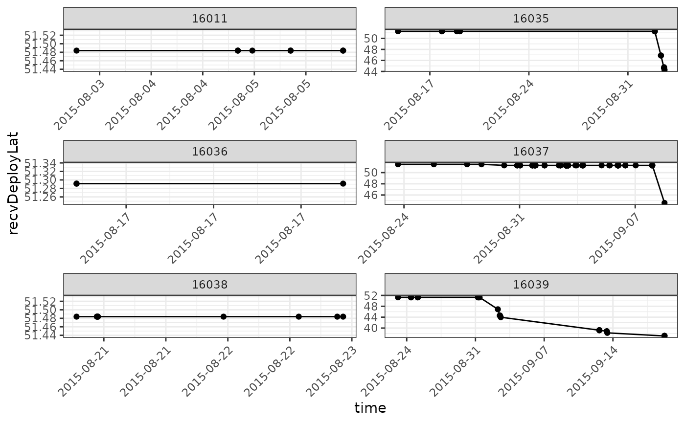
Although there don’t seem to be any immediate problems, let’s take a look at the tags showing up around 44 degrees during September. Let’s examine these tags in more detail by examining the runs in the data frame that are associated with detections in September.
tbl_alltags_sub %>%
  filter(motusTagID %in% c(16035, 16037, 16039),
         recvDeployLat < 44) %>%
  collect() %>%
  mutate(time = as_datetime(ts)) %>%
  filter(month(time) == 9) %>%
  group_by(recvDeployName, month = month(time), runLen) %>%
  summarize(n = length(time),
            n.tags = length(unique(motusTagID)),
            .groups = "drop") %>%
  arrange(runLen)
## # A tibble: 14 × 5
## recvDeployName month runLen n n.tags
## <chr> <dbl> <int> <int> <int>
## 1 Assateague State Park 9 6 6 1
## 2 FINWR 9 6 6 1
## 3 FINWR 9 10 10 1
## 4 FINWR 9 20 20 1
## 5 Prime Hook 9 23 23 1
## 6 BULL 9 24 24 1
## 7 Prime Hook 9 27 27 1
## 8 Bombay Hook 9 32 32 1
## 9 Prime Hook 9 32 32 1
## 10 Bombay Hook 9 36 36 1
## 11 BULL 9 38 38 1
## 12 Port Maitland 9 42 42 1
## 13 Bombay Hook 9 53 53 1
## 14 FINWR 9 73 73 1Since we have already filtered dubious detections, these remaining
ones don’t seem immediately unreliable (all with high
runLen). If you are interested, you can re-run the code
above, but on the full data frame
(tbl(sql_motus, "alltags")) containing run lengths of 2 or
3. You will see that there are likely false positive detections at these
sites, that were already eliminated by filtering.
Hypothetically, if we decided that those detections in September were
false positives, we could create a data frame that contains the
motusTagIDs and runIDs for them:
df_block_1 <- tbl_alltags_sub %>%
  filter(motusTagID %in% c(16035, 16037, 16039)) %>%
  collect() %>%
  mutate(time = as_datetime(ts)) %>%
  filter(month(time) == 9) %>%
  select(motusTagID, runID) %>%
  distinct() %>%
  collect()
Remove them from our plotting data frame:
And then plot our data again, having omitted those detections:
ggplot(data = filter(df_summary_sub,
                     motusTagID %in% c(16011, 16035, 16036, 16037, 16038, 16039)),
       aes(x = time, y = recvDeployLat)) +
  theme_bw() +
  theme(axis.text.x = element_text(angle = 45, vjust = 1, hjust = 1)) +
  geom_point() +
  geom_path() +
  facet_wrap(~ motusTagID, scales = "free", ncol = 2) +
  scale_x_datetime(date_labels = "%Y-%m-%d")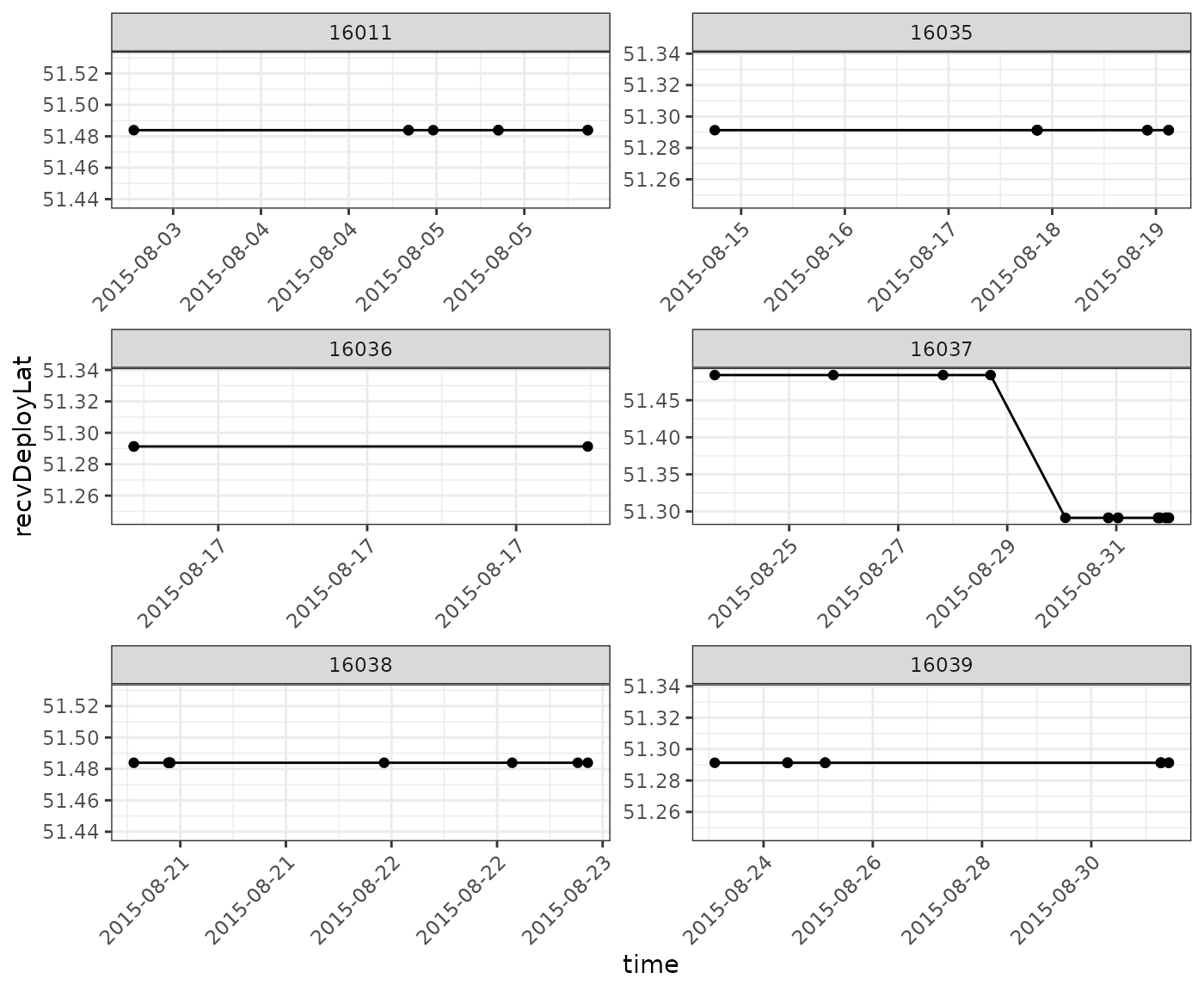
You are encouraged to explore the rest of the tags within this group, to determine if there are additional false positives.
Examining ambiguous detections
Before we go further, we need to check to see if any tags have ambiguous detections. If any do, we will need to explore them, and create additional filters to remove detections from our database.
Are any of your tags associated with ambiguous detections?
The clarify() function in the motus R
package provides a summary of ambiguities in the detections data. Each
ambigID refers to a selection of detections that could
belong to one or more (up to 6) motusTagIDs, which are
listed in the id1 to id6 columns:
clarify(sql_motus)## ambigID numHits id1 fullID1 id2
## 1 -337 4 10811 Niles#152:6.1@166.38(M.10811) 16011
## 2 -171 2074 22778 RBrownAMWO#308:5.3@166.38(M.22778) 22902
## 3 -134 22749 22905 SampleData#301:5.3@166.38(M.22905) 23319
## 4 -114 86 22897 SampleData#303.1:5.3@166.38(M.22897) 24298
## 5 -106 279 17021 Selva#172:6.1@166.38(M.17021) 17357
## 6 -56 5734 22867 SampleData#272.1:5.3@166.38(M.22867) 23316
## fullID2 id3 fullID3
## 1 SampleData#152:6.1@166.38(M.16011) NA <NA>
## 2 SampleData#308.1:5.3@166.38(M.22902) 24303 NEONICS#308:5.3@166.38(M.24303)
## 3 SampleData#301.1:5.3@166.38(M.23319) NA <NA>
## 4 NEONICS#303:5.3@166.38(M.24298) NA <NA>
## 5 SampleData#172:6.1@166.38(M.17357) NA <NA>
## 6 SampleData#272:5.3@166.38(M.23316) NA <NA>
## id4 fullID4 id5 fullID5 id6 fullID6 motusTagID tsStart tsEnd
## 1 NA NA NA NA NA NA NA NA NA
## 2 NA NA NA NA NA NA NA NA NA
## 3 NA NA NA NA NA NA NA NA NA
## 4 NA NA NA NA NA NA NA NA NA
## 5 NA NA NA NA NA NA NA NA NA
## 6 NA NA NA NA NA NA NA NA NAWe can see that there are six tags with ambiguous detections within
this data set. Detections associated with five of the six
ambigIDs could belong to one of two tags, and detections
associated with one ambigID (-171) could
belong to one of three tags. The fullID fields list the
project names associated with the duplicate tags (e.g., “SampleData”,
“Selva”, “Niles”), along with features of the tags (manufacturer tag ID,
burst, and transmit frequency).
Let’s get a data frame of these, and do some plots to see where there may be issues.
df_ambigTags <- tbl_alltags_sub %>%
  select(ambigID, motusTagID) %>%
  filter(!is.na(ambigID)) %>%
  distinct() %>%
  collect()
Using our df_summary, data frame we can filter these
detections. We also need to create new IDs showing links between
ambiguous and non-ambiguous detections of tags that have ambiguous
detections:
df_summary.ambig <- filter(df_summary, motusTagID %in% df_ambigTags$motusTagID) %>%
  mutate(ambig = !is.na(ambigID)) # Ambiguous or not? TRUE/FALSE

# to put all ambiguous tags from the same project on the same plot together, we
# need to create a new 'ambig tag' variable we call 'newID' that includes the
# multiple 'motusTagIDs' for each 'ambigID'

ambigTags2 <- tbl_alltags_sub %>%
  select(ambigID, motusTagID) %>%
  filter(!is.na(ambigID)) %>%
  distinct() %>%
  collect() %>%
  group_by(ambigID) %>%
  summarize(newID = paste(unique(ambigID), toString(motusTagID), sep = ": ")) %>%
  left_join(df_ambigTags, by = "ambigID")

# and merge that with 'df_summary'

df_summary.ambig <- left_join(df_summary.ambig, ambigTags2, by = "motusTagID") %>%
  arrange(time)
Plot the results! We’ll add some information to the plot, showing where (in time) the tags are actually ambiguous. We can then inspect the overall plots (or portions of them) to determine if we can contextually unambiguously assign a detection of an ambiguous tag to a single deployment.
ggplot(data = df_summary.ambig,
       aes(x = time, y = recvDeployLat, colour = ambig)) +
  theme_bw() +
  theme(axis.text.x = element_text(angle = 45, vjust = 1, hjust = 1)) +
  geom_point() +
  geom_path() +
  facet_wrap(~ newID, scales = "free", ncol = 2)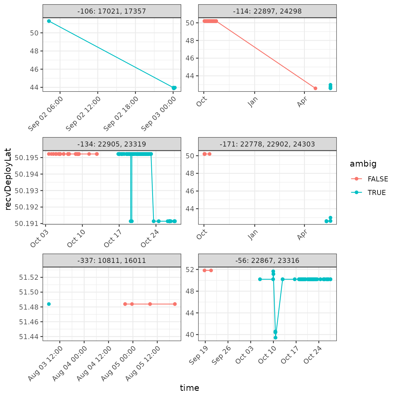
Let’s deal with the easy ones first.
ambigID -337: motusTagIDs 10811 and
16011
tbl_alltags_sub %>%
  filter(ambigID == -337) %>%
  count(motusTagID, tagDeployStart, tagDeployEnd, tagDepLat, tagDepLon) %>%
  collect() %>%
  mutate(tagDeployStart = as_datetime(tagDeployStart),
         tagDeployEnd = as_datetime(tagDeployEnd))
## # A tibble: 2 × 6
## motusTagID tagDeployStart tagDeployEnd tagDepLat tagDepLon n
## <int> <dttm> <dttm> <dbl> <dbl> <int>
## 1 10811 2014-10-28 07:00:00 2015-08-03 07:00:00 39.1 -74.7 4
## 2 16011 2015-08-02 11:39:59 2015-12-17 11:39:59 51.5 -80.4 4We can see from the plot that ambiguous tag -337 is ambiguous only at the beginning of the deployment.
We can see from the summary of the tag deployment data that there
were only 4 detections, at the exact latitude of deployment of tag
16011, and just before the non-ambiguous detections of
motusTagID 16011. So the issue here is simply that the tail
end of the deployment of tag 10811 slightly overlaps with the deployment
of tag 16011. We can confidently claim these detections as belonging to
motusTagID 16011, and remove the ambiguous detections assigned to the
other tag.
We’ll create another data frame to keep track of these runs.
# we want the detections associated with the motusTagID that we want to
# ultimately REMOVE from the data frame
df_block_2 <- tbl_alltags_sub %>%
  filter(ambigID == -337,
         motusTagID == 10811) %>%
  select(motusTagID, runID) %>%
  distinct() %>%
  collect()
ambigID -134: motusTagIDs 22905 and
23319
tbl_alltags_sub %>%
  filter(ambigID == -134) %>%
  collect() %>%
  mutate(tagDeployStart = as_datetime(tagDeployStart),
         tagDeployEnd = as_datetime(tagDeployEnd),
         month = month(as_datetime(ts))) %>%
  count(motusTagID, tagDeployStart, tagDeployEnd,
           tagDepLat, tagDepLon, month)
## # A tibble: 2 × 7
## motusTagID tagDeployStart tagDeployEnd tagDepLat tagDepLon month
## <int> <dttm> <dttm> <dbl> <dbl> <dbl>
## 1 22905 2016-10-01 16:00:00 2017-06-12 16:00:00 50.2 -63.7 10
## 2 23319 2016-10-15 16:00:00 2017-06-26 16:00:00 50.2 -63.7 10
## # ℹ 1 more variable: n <int>Here we have a similar situation, but one that is a bit more complex. Two identical tags were deployed at the same location, shortly after one another. Let’s examine a simple plot.
df_plot <- tbl_alltags_sub %>%
  filter(motusTagID %in% c(22905, 23319)) %>%
  collect() %>%
  mutate(time = as_datetime(ts))

ggplot(data = df_plot,
       aes(x = time, y = sig, group = recvDeployName, colour = recvDeployName)) +
  geom_point() +
  theme_bw() +
  labs(x = "Time", y = "Signal strength") +
  facet_grid(recvDeployLon ~ .)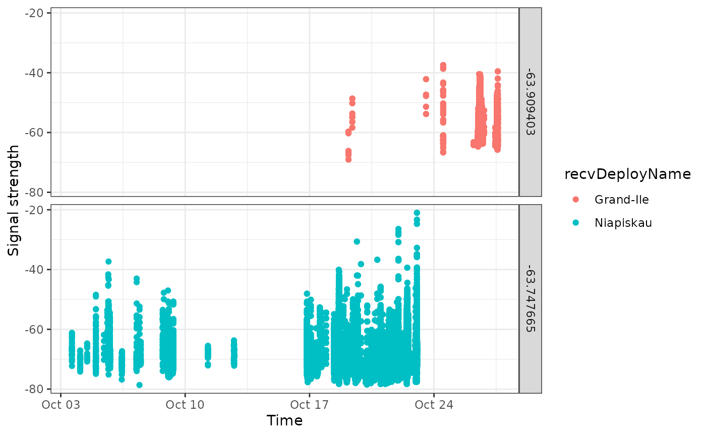
It appears that these are overlapping detections, at two sites in proximity to one another. Additional information from the field researchers may enable us to disentangle them, but it is not clear from the data.
We will therefore remove all detections of this ambiguous tag from
the database. To do so, we collect the motusTagIDs that we
want to remove.
df_block_3 <- tbl_alltags_sub %>%
  filter(ambigID == -134) %>%
  select(motusTagID, runID) %>%
  distinct() %>%
  collect()
ambigID -171: motusTagIDs 22778,
22902 and 22403
The ambiguous detections for this tag, which occur in the Great Lakes
region, could also belong to motusTagID 22778 from the
RBrownAMWO project or motusTagID 24303 from the Neonics
project. Let’s take a closer look at these detections.
First, find the deployment dates and locations for each tag.
tbl_alltags_sub %>%
  filter(ambigID == -171) %>%
  filter(!is.na(tagDeployStart)) %>%
  select(motusTagID, tagProjID, start = tagDeployStart, end = tagDeployEnd,
         lat = tagDepLat, lon = tagDepLon, species = speciesEN) %>%
  distinct() %>%
  arrange(start) %>%
  collect() %>%
  mutate(start = as_datetime(start),
         end = as_datetime(end))
## # A tibble: 3 × 7
## motusTagID tagProjID start end lat lon
## <int> <int> <dttm> <dttm> <dbl> <dbl>
## 1 22902 176 2016-10-01 16:00:00 2017-06-12 16:00:00 50.2 -63.7
## 2 22778 82 2016-10-21 00:00:00 2018-09-09 00:00:00 45.1 -67.3
## 3 24303 146 2017-05-10 22:30:59 2017-06-30 22:30:59 42.6 -80.5
## # ℹ 1 more variable: species <chr>Then plot the ambiguous detections by date and receiver.
df_ambgi_171 <- filter(tbl_alltags_sub, ambigID == -171) %>%
  collect() %>%
  mutate(time = as_datetime(ts),
         date = as_date(time))

ggplot(data = df_ambgi_171, aes(x = time, y = sig, colour = as.factor(port))) +
  theme_bw() +
  theme(axis.text.x = element_text(angle = 45, vjust = 1, hjust = 1)) +
  geom_point() +
  geom_smooth(method = "loess", se = FALSE) +
  facet_wrap(date ~ recvDeployName, scales = "free_x")
## `geom_smooth()` using formula = 'y ~ x'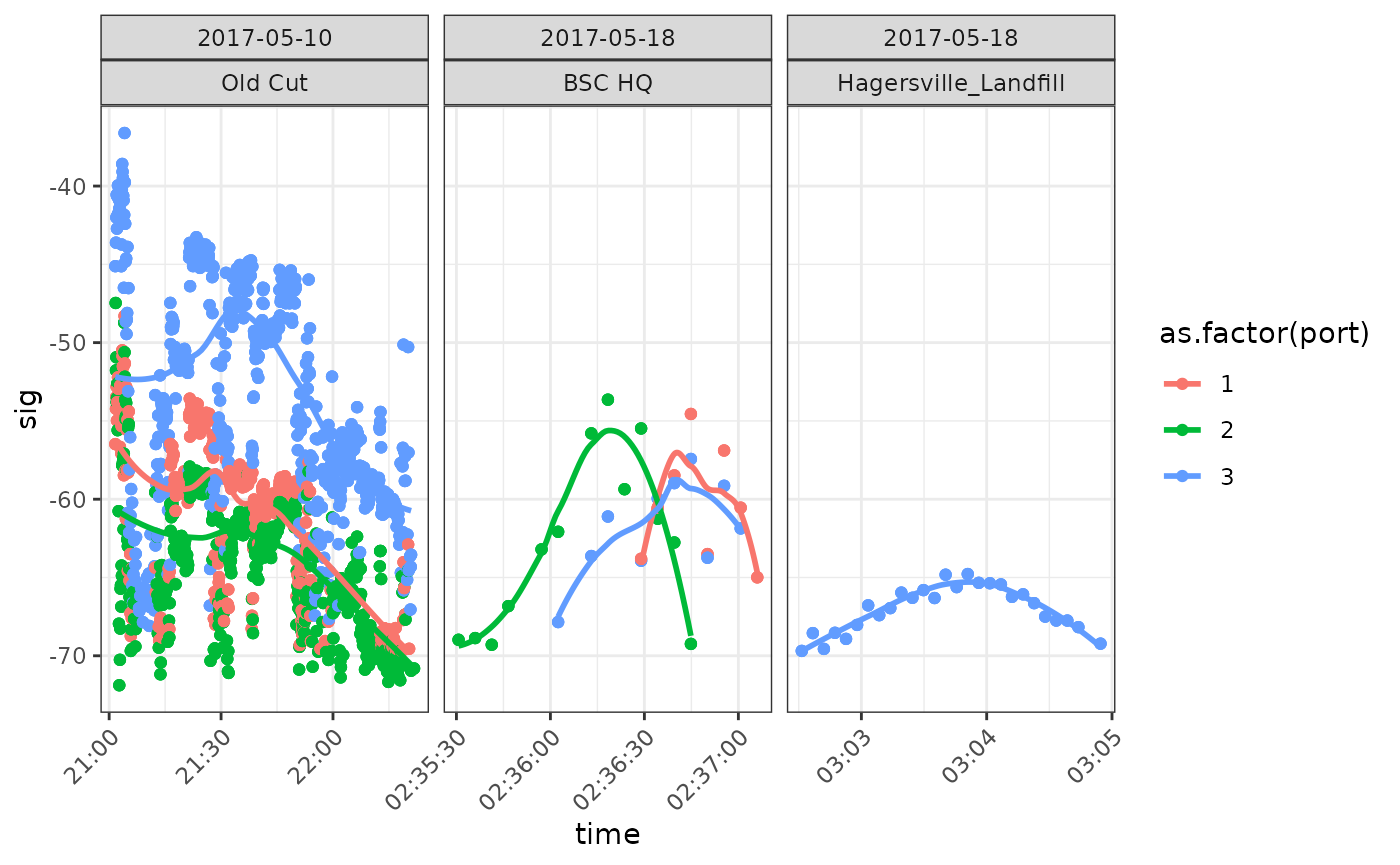
We see that there are a large number of ambiguous detections on 10
May 2017 at Old Cut (Long Point, Lake Erie, Ontario), consistent with a
bird ‘hanging around’. These are almost certainly detections of
motusTagID ‘24303’ which was deployed at Old Cut on 10 May
2017. Subsequent detections on the 18th of May are near Old Cut (Bird
Studies Canada HQ, Port Rowan, Ontario), and then a location to the
North of Old Cut (Hagersville, Ontario). These detections are consistent
with a bird departing on migration. Note in particular the pattern in
the latter two panels of increasing then decreasing signal strength
which indicates a bird is flying through the beam of an antenna.
These detections belong to another project, so we simply remove all detections of that ambiguous tag from our database.
df_block_4 <- tbl_alltags_sub %>%
  filter(ambigID == -171) %>%
  select(motusTagID, runID) %>%
  distinct() %>%
  collect()
ambigID -114: motusTagIDs 22897 and
24298
Next we look at the ambiguities for ambiguous tag -114.
tbl_alltags_sub %>%
  filter(ambigID == -114) %>%
  filter(!is.na(tagDeployStart)) %>%
  select(motusTagID, tagProjID, start = tagDeployStart, end = tagDeployEnd,
         lat = tagDepLat, lon = tagDepLon, species = speciesEN) %>%
  distinct() %>%
  arrange(start) %>%
  collect() %>%
  mutate(start = as_datetime(start),
         end = as_datetime(end))
## # A tibble: 2 × 7
## motusTagID tagProjID start end lat lon
## <int> <int> <dttm> <dttm> <dbl> <dbl>
## 1 22897 176 2016-10-01 16:00:00 2017-06-12 16:00:00 50.2 -63.7
## 2 24298 146 2017-05-10 03:00:00 2017-06-30 03:00:00 42.6 -80.5
## # ℹ 1 more variable: species <chr>We again subset these detections and plot them. An initial plot suggested that all of the detections represent a migratory flight, so we construct a somewhat different plot from the one above that emphasizes this behaviour better.
df_ambgi_114 <- tbl_alltags_sub %>%
  filter(ambigID == -114) %>%
  collect() %>%
  mutate(LatLonStationName = paste(recvDeployLat, recvDeployLon,
                                   recvDeployName, sep=": "),
         time = as_datetime(ts))

ggplot(data = df_ambgi_114, aes(x = time, y = sig, colour = LatLonStationName)) +
  geom_point() +
theme_bw() 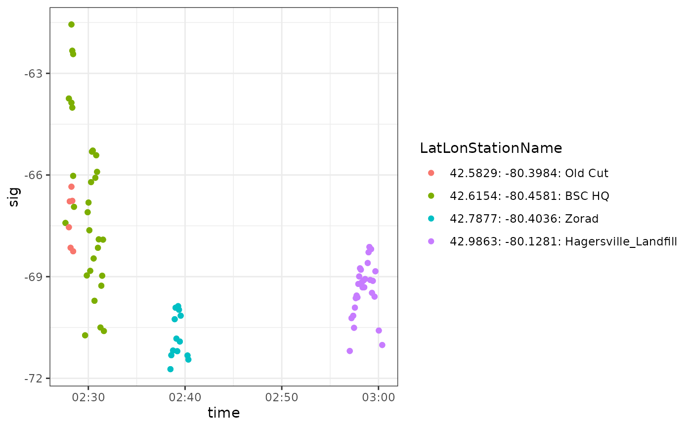
Notice that these detections are consistent with a migratory departure from the Long Point area (Old Cut Field Station, Lake Erie, Ontario) about a week after the ambiguous tag 24298 was deployed at the same location. This again suggests that these ambiguous detections can be removed from our data because they belong to another project.
df_block_5 <- tbl_alltags_sub %>%
  filter(ambigID == -114) %>%
  select(motusTagID, runID) %>%
  distinct() %>%
  collect()
ambigID -106: motusTagIDs 17021 and
17357
These two tags pose an interesting problem. There is only a short period of overlap, between mid-August 2015 and mid-September. One individual is a Grey-cheeked Thrush, tagged in Colombia, the other a White-rumped Sandpiper, associated with the sample project.
tbl_alltags_sub %>%
  filter(ambigID == -106) %>%
  filter(!is.na(tagDeployStart)) %>%
  select(motusTagID, tagProjID, start = tagDeployStart, end = tagDeployEnd,
         lat = tagDepLat, lon = tagDepLon, species = speciesEN) %>%
  distinct() %>%
  arrange(start) %>%
  collect() %>%
  mutate(start = as_datetime(start),
         end = as_datetime(end))
## # A tibble: 2 × 7
## motusTagID tagProjID start end lat lon
## <int> <int> <dttm> <dttm> <dbl> <dbl>
## 1 17021 57 2015-04-30 05:00:00 2015-09-14 05:00:00 11.1 -74.1
## 2 17357 176 2015-08-11 07:20:00 2015-12-26 07:20:00 51.5 -80.4
## # ℹ 1 more variable: species <chr>We plot the ambiguous detections by date to examine the period of overlap.
df_ambgi_106 <- tbl_alltags_sub %>%
  filter(ambigID == -106) %>%
  collect() %>%
  mutate(time = as_datetime(ts),
         date = as_date(time),
         col = paste(recvDeployLat, recvDeployLon, recvDeployName, sep = ": "))

ggplot(data = df_ambgi_106, aes(x = time, y = sig, colour = col)) +
  theme_bw() +
  geom_point() +
  scale_colour_discrete(name = "Lat/Lon and\nStation Name") +
  facet_wrap(~ date, scales = "free_x")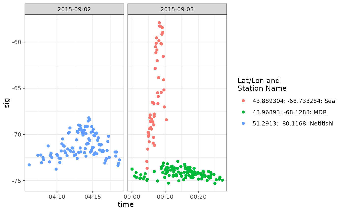
Both sets of detections are long run lengths, and look valid
(increasing then decreasing signal strength). They are about a day
apart, and so it is possible they represent two different birds, or the
departure flight of the White-rumped Sandpiper from its staging ground.
Let’s use the siteTrans() function to examine the flight
from Netitishi to MDR/Seal (in the Gulf of Maine).
df_ambgi_106 %>%
  filter(motusTagID == 17021) %>% # just pick one of the two ambiguous IDs
  siteTrans() %>%
  filter(rate < 60) %>% # remove the simultaneous detections from Seal and MDR
  mutate(total_time = as.numeric(round(seconds_to_period(tot_ts)))) %>%
  select(start = recvDeployName.x, end = recvDeployName.y,
         date = ts.x, `rate(m/s)` = rate,
         dist, total_time = total_time, bearing)
## # A tibble: 1 × 7
## start end date `rate(m/s)` dist total_time bearing
## <chr> <chr> <dttm> <dbl> <dbl> <dbl> <dbl>
## 1 Netitishi_51.… MDR_… 2015-09-02 04:18:42 17.1 1.21e6 70879 128.These detections are >1200 km distant from one another, but the
flight speed (17 m/s) is consistent with a White-rumped Sandpiper. Given
that the Gray-cheeked Thrush tag was near the end of its expected
lifetime, we can reasonably claim these detections for our project, and
remove the ambiguous detections associated with motusTagID
17021.
df_block_6 <- tbl_alltags_sub %>%
  filter(ambigID == -106, motusTagID == 17021) %>%
  select(motusTagID, runID) %>%
  distinct() %>%
  collect()
ambigID -56: motusTagIDs 22867 and
23316
These two tags were also both deployed by the same project.
tbl_alltags_sub %>%
  filter(ambigID == -56) %>%
  filter(!is.na(tagDeployStart)) %>%
  select(motusTagID, tagProjID, start = tagDeployStart, end = tagDeployEnd,
         lat = tagDepLat, lon = tagDepLon, species = speciesEN) %>%
  distinct() %>%
  arrange(start) %>%
  collect() %>%
  mutate(start = as_datetime(start),
         end = as_datetime(end))
## # A tibble: 2 × 7
## motusTagID tagProjID start end lat lon
## <int> <int> <dttm> <dttm> <dbl> <dbl>
## 1 22867 176 2016-09-06 15:35:00 2017-05-18 15:35:00 51.8 -80.7
## 2 23316 176 2016-10-02 16:00:00 2017-06-13 16:00:00 50.2 -63.7
## # ℹ 1 more variable: species <chr>Tag 23316 was deployed by the James Bay Shorebird Project (sample project) about three weeks after tag 22867, which was deployed from a location far to the west.
df_ambgi_56 <- tbl_alltags_sub %>%
  filter(ambigID == -56) %>%
  collect() %>%
  mutate(sig = ifelse(sig > 0, sig * -1, sig),
         time = as_datetime(ts),
         col = paste(recvDeployLat, recvDeployLon, recvDeployName, sep=": "))

ggplot(data = df_ambgi_56, aes(x = time, y = recvDeployLon, colour = col)) +
  theme_bw() +
  geom_point() +
scale_colour_discrete(name="Lat/Lon and\nStation Name") 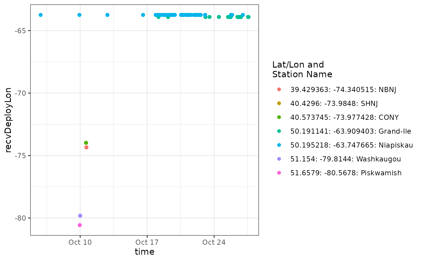
We can see from the plot that a tag is detected consistently near
longitude -65, which is near the deployment location for
motusTagID 23316 and after it’s deployment start date, it
was also present at -65 during and after detections far to the west.
It’s likely all the detections at -65 belong to motusTagID
23316, but it is also clear that anything informative about this
ambiguity occurs between about 9-11 October, so let’s zoom in on that
part of the data set.
time.begin <- "2016-10-06 00:00:00"
time.end <- "2016-10-12 23:00:00"

ggplot(data = filter(df_ambgi_56, time > time.begin, time < time.end),
       aes(x = time, y = recvDeployLon, colour = col)) +
  theme_bw() +
  geom_point() +
scale_colour_discrete(name = "Lat/Lon and\nStation Name") 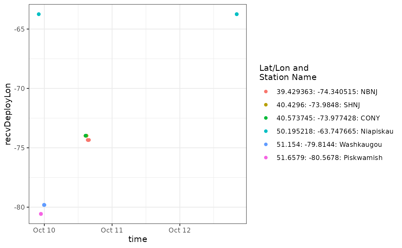
We can see that the ambiguous tag was detected consistently at
Niapiskau and Grand Ile before and after the period when it was also
detected to the north and west (at Washkaugou and Piskwamish) and then
to the south (NBNJ, SHNJ, and CONY). We can look at this transition by
filtering out the portion of the data not near Niapiskau, and again
using the siteTrans() function from the motus
package.
# other tag is a duplicate
df_56_tmp <- filter(df_ambgi_56, !(recvDeployLat == 50.2), motusTagID == 22867)

siteTrans(df_56_tmp) %>%
  filter(rate < 60) %>% # get rid of simultaneous detections
  mutate(total_time = as.numeric(round(seconds_to_period(tot_ts)))) %>%
  select(start = recvDeployName.x,
         end = recvDeployName.y,
         date = ts.x, `rate(m/s)` = rate,
         dist, total_time = total_time, bearing)
## # A tibble: 11 × 7
## start end date `rate(m/s)` dist total_time bearing
## <chr> <chr> <dttm> <dbl> <dbl> <dbl> <dbl>
## 1 Piskwamish_5… Wash… 2016-10-09 22:49:59 20.4 7.68e4 3767 137.
## 2 Washkaugou_5… SHNJ… 2016-10-10 00:00:42 24.3 1.27e6 52386 157.
## 3 NBNJ_39.4, -… Niap… 2016-10-10 15:47:37 7.74 1.46e6 188426 31.4
## 4 Niapiskau_50… Gran… 2016-10-18 04:22:02 43.5 1.16e4 266 -92.2
## 5 Grand-Ile_50… Niap… 2016-10-18 04:29:12 0.728 1.16e4 15887 87.7
## 6 Grand-Ile_50… Niap… 2016-10-19 04:34:04 0.531 1.16e4 21758 87.7
## 7 Niapiskau_50… Gran… 2016-10-23 01:39:14 5.55 1.16e4 2084 -92.2
## 8 Grand-Ile_50… Niap… 2016-10-25 17:57:52 19.3 1.16e4 600 87.7
## 9 Niapiskau_50… Gran… 2016-10-25 21:13:49 0.243 1.16e4 47541 -92.2
## 10 Grand-Ile_50… Niap… 2016-10-26 19:43:34 0.758 1.16e4 15254 87.7
## 11 Niapiskau_50… Gran… 2016-10-27 00:03:21 0.246 1.16e4 46941 -92.2The bird made a 14.5 hour (52386/60/60) flight between Washkaugou and
SHNJ at a rate of 24 m/s, which is plausible. The researchers involved
may have other data to support or refute the inference (e.g. an actual
sighting of the Red Knot still in Niapiskau after this flight was
recorded) but it seems likely that while one tag remained at sites
around longitude -65, another tag made the above migratory
flights.
We can make another more detailed plot of signal strength to examine
these potential migratory flights more closely:
df_56_tmp <- tbl_alltags_sub %>%
  filter(ambigID == -56, recvDeployLon < -70) %>%
  collect() %>%
  mutate(time = as_datetime(ts),
         date = as_date(time),
         col = paste(recvDeployLat, recvDeployLon, recvDeployName, sep = ": "))

ggplot(data = df_56_tmp, aes(x = time, y = sig, colour = col)) +
  theme_bw() +
  geom_point() +
  scale_colour_discrete(name = "Lat/Lon and\nStation Name") +
  facet_wrap(~ date, scales = "free_x")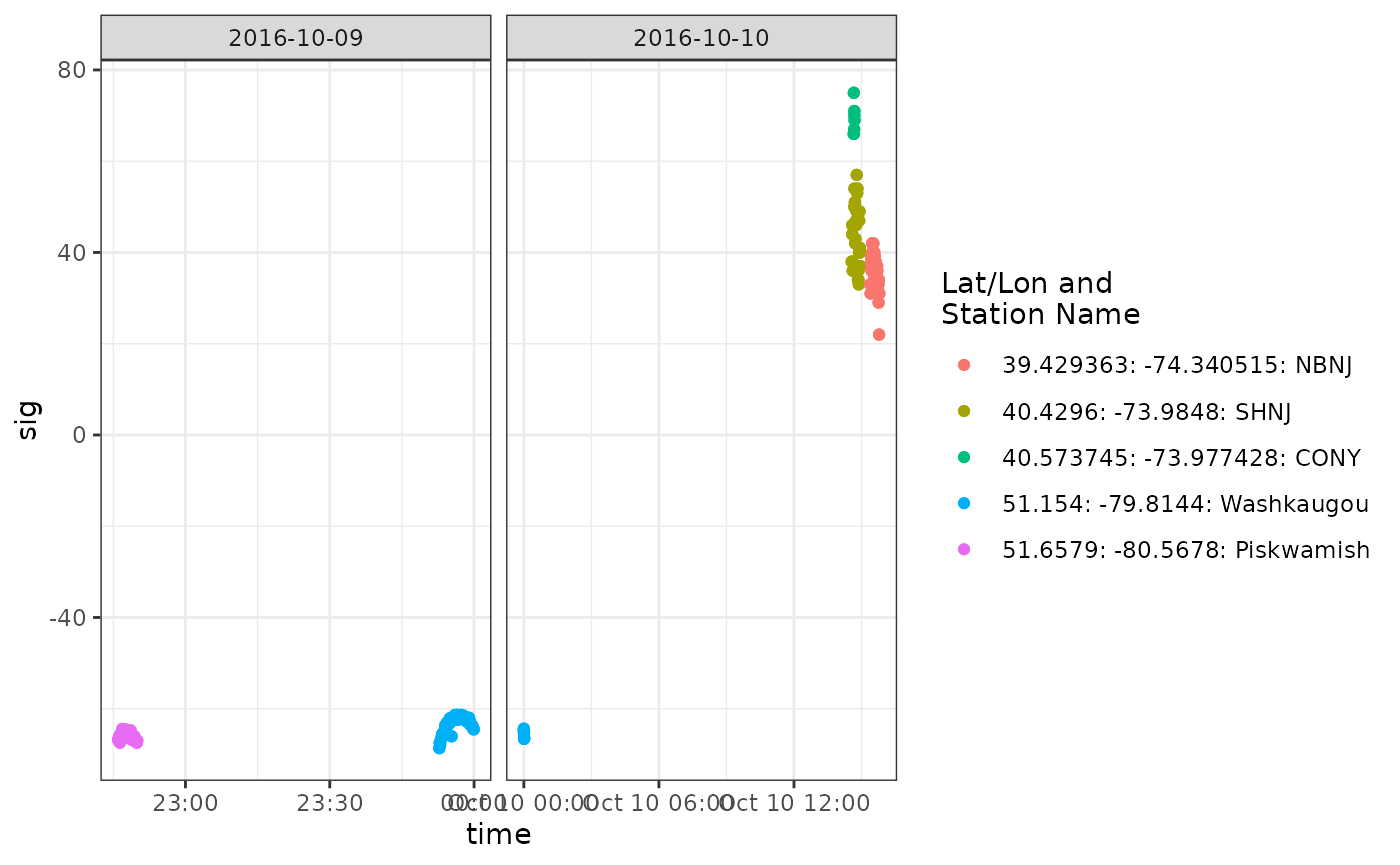
These look like typical fly-by patterns of increasing and then
decreasing signal strength.
This, coupled with overall detection patterns and knowledge of the
species, leads us to believe that the ambiguous detections can be
reasonably divided between the two individuals; one detected
consistently around longitude -65 (23316), and the other migrating SW
during the same period (22867).
To address this problem, we need to create two filters: one that
excludes ambiguous detections of tag 22867, and one that excludes some
detections of 23316. In this instance, we can do this most easily by
filtering on motusTagID and
recvDeployName.
Tag 23316 was only ever at “Grand-Ile”, “Niapiskau”, and tag 22867 was never detected at those sites. So we exclude all detections not at “Grand-Ile”, “Niapiskau” for motusTag 23316, and do the opposite for tag 22867.
df_block_7 <- tbl_alltags_sub %>%
  filter(ambigID == -56,
         motusTagID == 23316,
         !(recvDeployName %in% c("Grand-Ile", "Niapiskau"))) %>%
  select(motusTagID, runID) %>%
  distinct() %>%
  collect()

df_block_8 <- tbl_alltags_sub %>%
  filter(ambigID == -56,
         motusTagID == 22867,
         recvDeployName %in% c("Grand-Ile", "Niapiskau")) %>%
  select(motusTagID, runID) %>%
  distinct() %>%
  collect()
Checking validity of short runs
At the beginning of this chapter, we removed all short/noisy
detections with a motusFilter of 0, because they are
considered to have a high probability of being false positive. Now that
we’ve cleaned the data, and are confident in the detections that remain,
you might at this point decide to go back and take a closer look at
those omitted detections. You could do this, for example, by re-running
the various plots described in this chapter (begin with lat/lon by time
plots), to see if any of those detections make sense in the context of
where the true detections lie. It is up to the user to decide which
detections are reasonable in terms of the biology and behaviour of each
tagged individual.
Filtering the data
Filter and save to RDS
To filter the data, we can omit rows in the df_block
data frames from the original data using a anti_join(),
which removes rows from x (tbl_alltags_sub)
which are present in y (df_block). First we
will combine all of our df_block data frames into a single
data frame:
df_block_all <- bind_rows(df_block_0, df_block_2, df_block_3,
                          df_block_4, df_block_5, df_block_6, df_block_7,
                          df_block_8)

df_alltags_sub <- tbl(sql_motus, "alltags") %>%
  collect() %>%
  anti_join(df_block_all, by = c("runID", "motusTagID"))
Now save the local data frame as an RDS file, for use in the next
chapter. Recall from Exporting detections
in Chapter 3 that the RDS format preserves the R data structure,
including time stamps. The other benefit of saving to RDS is that you
have the output from a given workflow saved as a flat file, which you
can access again with a simple readRDS() statement.
saveRDS(df_alltags_sub, file = "./data/dfAlltagsSub.rds")And to read the data in again:
df_alltags_sub <- readRDS("./data/dfAlltagsSub.rds")Save a custom filter in the motus database, and apply it to the data
As an alternative to saving your data as an RDS file, the Motus R
package offers functionalities to save your filters directly within your
.motus file. Once they are saved in your database, you can
do the type of anti_join() as above without having to rely
on dataframes or an RDS file to store your data. To learn more about the
functions available to work with Motus filters, see the filtering
section in the function
reference for more details.
df_block_all <- bind_rows(df_block_0, df_block_2, df_block_3,
                          df_block_4, df_block_5, df_block_6, df_block_7,
                          df_block_8) %>%
  mutate(probability = 0)

# create a new filter with name filtAmbigFalsePos and populate it with df_block_all
tbl_filter <- writeRunsFilter(sql_motus, "filtAmbigFalsePos",
                              df = df_block_all, delete = TRUE)
## Filter records savedNow you can obtain a table object where the filtered records from
tbl_filter have been removed:
Next Chapter 6 - Exploring detections data (Explore all articles)